
Important Definitions in Linear programming Model:
The following important definitions in Linear programming Model are necessary for understanding and developing the theory that follows:
Solution of LPP:
A set of variables {x1, x2, x3, …, xn, s1, s2, …, sm} is called a solution of the linear programming problem if it satisfies the set of constraints.
Feasible Region:
The area containing all the feasible solutions to the LPP is called a feasible region in a graph. In other words, it is a region in which all constraints and non-negativity conditions hold good.
In other words, the collection of all feasible solutions is called the feasible region.
Example 1:
Consider the following LPP:
Maximize Z = 3x1+ 5x2
Subject to
x1≤ 4
2x2≤ 12
3x1+2x2 ≤ 18
and
x1 ≥ 0, x2 ≥ 0.
Draw the feasible region for this LPP.
Solution:
Draw the graphs of all constraints and non-negativity restrictions, as shown follows.
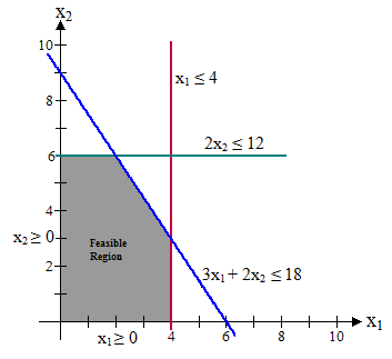
The feasible region in this example is the entire shaded area of this Figure, which is a set of permissible values of (x1, x2).
Feasible Solution:
A set of variables {x1, x2, x3, …, xn, s1, s2, …, sm} is called a feasible solution if these variables satisfy all constraints and non-negative restrictions. In other words, a feasible solution is one that satisfies all of the constraints and non-negative restrictions.
It is possible for a problem to have no feasible solutions.
Infeasible Solution: An infeasible solution is one that contradicts at least one constraint, that is, that fails to satisfy at least one constraint.
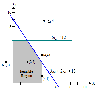
In the above Figure 1 of Example 1, the points (2,3) and (4,1) are feasible solutions, while the points (−1,3) and (4,4) are infeasible solutions, as shown follows:
Optimal solution:
A feasible solution with the most favourable objective function value is called an optimal solution.
- If the objective function is to be maximised, the most favourable value is the largest value;
- if the objective function is to be minimised, the most favourable value is the smallest value.
Consider the LPP from Example 1:
Maximize Z = 3x1+ 5x2
Subject to
x1≤ 4
2x2≤ 12
3x1+2x2 ≤ 18
and
x1 ≥ 0, x2 ≥ 0.
Find the optimal solution for this LPP.
Solution:
First, draw the feasible region for this LPP as shown in Figure-1. The final step is to find the point in this feasible region that gives the maximum value of Z = 3x1+5x2. Start by trial and error to know how to perform this step efficient manner.
Try, for example, Z = 10 = 3x1+5x2.
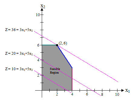
By drawing the line Z=10=3x1+5x2, we can see that there are many points on this line that lies within the region.
After achieving perspective by trying this arbitrarily chosen value of Z = 10, we should next try a larger arbitrary value of Z, such as Z = 20 = 3x1+5x2. Again, Figure-3 reveals that a segment of the line Z = 20 = 3x1+5x2 lies within the region so that the maximum permissible value of Z must be at least 20.
Now notice in Figure-3 that the two lines just constructed are parallel. These observations imply that our trial-and-error procedure for constructing lines in Figure-3 involves nothing more than drawing a family of parallel lines containing at least one point in the feasible region and choosing the line that corresponds to the maximum value of Z.
Figure-3 shows that this line passes through the point (2,6), indicating that the optimal solution is, x1=2, and x2=6. The value of (x1, x2) that maximizes the objective function Z = 3x1+5x2 is (2,6). The equation of this line is Z= 3x1+5x2 = 3(2)+5(6)=36, indicating that the optimal value of Z is Z=36.
Having seen the trial-and-error procedure for finding the optimal point (2,6), you now can streamline this approach for other problems. Instead of drawing several parallel lines, a single line with a ruler is sufficient to establish the slope. Then move the ruler with a fixed slope through the feasible region in the direction of improving Z.
The example has exactly one optimal solution, (x1,x2)=(2,6), which is a CPF (corner-point feasible) solution.
Read Also: Graphical Method for solving LPP
♦ There may be multiple optimal solutions to a problem:
There will be an infinite number of optimal solutions to any problem with multiple optimal solutions, each with the same optimal value of the objective function.
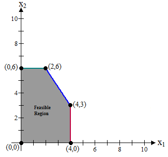
Example 2:
Consider the following LPP:
Maximize Z = 3x1+ 2x2
Subject to
x1 ≤ 4
2x2≤ 12
3x1+ 2x2 ≤ 18
and
x1≥ 0, x2≥ 0.
Find the optimal solution for this LPP.
Solution:
The graphical solution for this LPP is shown in the following Figure:

Here, every point on the darker blue line segment connecting (2,6) and (4,3) would be optimal, each with Z = 3x1+2x2 = 18.
Here, two of these optimal solutions: (2,6) and (4,3); are CPF (corner-point feasible) solutions.
♦ It is possible for a problem to have no optimal solutions:
This occurs only,
Case-1: If it has no feasible solutions, or
Case-2: If it has an unbounded Z, that is, the constraints do not stop the objective function’s value (Z) from improving indefinitely in either a positive or negative direction.
Case 1: If it has no feasible solutions.
Example 3:
Consider the following LPP:
Maximize Z = 3x1+5x2
Subject to
x1≤ 4
2x2≤ 12
3x1+2x2 ≤ 18
3x1+5x2 ≥ 50
and
x1 ≥ 0, x2 ≥ 0.
Find the optimal solution for this LPP.
Solution:
The graphical solution for this LPP is shown in the following Figure:
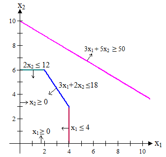
This LPP has no feasible solutions, and so this LPP has no optimal solutions.
Case 2: If it has an unbounded Z, that is, the constraints do not stop the objective function’s value (Z) from improving indefinitely in either a positive or negative direction.
Unbounded Solution:
An unbounded solution is one in which the value of the objective function can be increased or decreased indefinitely.
Example 4:
Consider the following LPP:
Maximize Z = 3x1+5x2
Subject to x1 ≤ 4
and x1 ≥ 0, x2 ≥ 0.
Find the optimal solution for this LPP.
Solution:
The graphical solution for this LPP is shown in the following Figure:
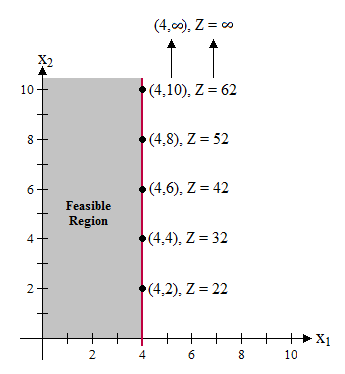
This LPP has no optimal solutions, if the only constraint were x1 ≤ 4, because x2 then could be increased infinitely in the feasible region without ever reaching the maximum value of Z = 3x1+ 5x2. In this case, the solution of this LPP is an unbounded solution.
Corner Point Feasible (CPF) solution:
A corner-point feasible (CPF) solution is a solution that lies at a corner of the feasible region. In other words, it is a feasible solution that does not lie on any line segment connecting two other feasible solutions.
Consider the Example 1:
Given LPP is:
Maximize Z = 3x1+5x2
Subject to
x1 ≤ 4
2x2≤12
3x1+2x2≤18
and
x1 ≥ 0, x2 ≥ 0.
Find the CPF solutions for this LPP.
The following figure highlights the five CPF solutions for this Example 1. The five dots are the five CPF solutions, as shown follows.
Relationship between optimal solutions and CPF solutions:
Consider any linear programming problem with feasible solutions and a bounded feasible region. The problem must possess CPF solutions and at least one optimal solution. Furthermore, the best CPF solution must be an optimal solution. Thus, if a problem has exactly one optimal solution, it must be a CPF solution. If the problem has multiple optimal solutions, at least two must be CPF solutions.
(Source – Various books from the college library)
Copyrighted Material © 2019 - 2024 Prinsli.com - All rights reserved
All content on this website is copyrighted. It is prohibited to copy, publish or distribute the content and images of this website through any website, book, newspaper, software, videos, YouTube Channel or any other medium without written permission. You are not authorized to alter, obscure or remove any proprietary information, copyright or logo from this Website in any way. If any of these rules are violated, it will be strongly protested and legal action will be taken.


Be the first to comment