Graphical Method for Solving LPP

Graphical method for solving LPP:

Simple linear programming problems of two variables can be easily solved by the graphical method. The outlines of the graphical method for solving lpp are as follows:

Step-1:

Consider each inequality-constraint as an equation.

Step-2:

Sketch the graph of each equation, because each one will represent a straight line geometrically.

Step-3:

Shade the feasible region. Each point on the line will satisfy the line’s equation.

• If the inequality constraint corresponding to that line is ‘≤’ then the region below the line lying in the first quadrant is shaded.
• If the inequality constraint corresponding to that line is ‘≥’ then the region above the line lying in the first quadrant is shaded.
• All points in the common region will satisfy all of the constraints at the same time.
• Thus obtained common region is known as the feasible region.

Step-4:

Find the optimum solution in the feasible region.

• To determine the optimum point, first, locate the corner points on the graph or find them by solving the concerned linear equations taken two at a time.
• Then, calculate the value of the objective function at each corner point.
• The corner at which the objective function is optimum (maximum or minimum), will give the optimum solution of the LPP.

Utility of Graphical Method for Solving LPP:

1. If there are only two variables, we can use a graphical method to solve LPP.

2. When there are two variables in the problem, we can refer to them as x₁ and x₂, and we can do most of the analysis on a two-dimensional graph.

3. Another advantage of the graphical approach is its visual nature.

4. Graphical methods provide us with a picture to go with the algebra of linear programming, and the picture can anchor our understanding of basic definitions and possibilities.

For these reasons, the graphical approach serves as an excellent foundation for working with linear programming concepts.

Example:

Solve the following LPP by the graphical method:

Maximize Z = 40x + 30y

Subject to

2x + y ≤ 16

  x + y ≤ 10

and,

x, y ≥ 0.

Solution:

To solve this linear programming problem, apply the following steps:

STEP 1: Sketch the system of inequalities.

• The restrictions x ≥ 0 means from the y-axis to the right, and y ≥ 0 means from the x-axis upward, so shaded only the first quadrant.

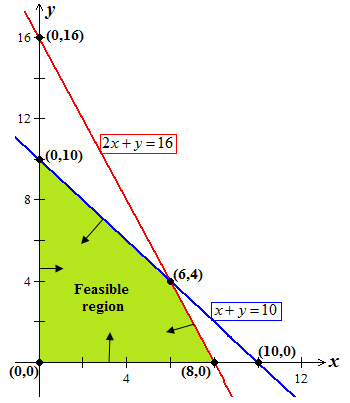
• First draw the line: 2x + y = 16, to sketch the graph of 2x + y ≤ 16.

Put x=0 into 2x + y = 16 and solve for y. So we get, y=16 at x=0, that is, the point (x, y) = (0, 16).

Put y=0 into 2x + y = 16 and solve for x. So we get, x=8 at y=0, that is, the point (x, y) = (8, 0).

Plot (0, 16) and (8, 0). Draw the line passing through these points. This line represents 2x + y = 16 as shown by the red colour in the following figure.

The constraint 2x + y ≤ 16 has ‘≤’ then shade the region below the line 2x + y = 16 lying in the first quadrant.

• Next draw the line: x + y = 10, to sketch the graph of x + y ≤ 10.

Put x=0 into x + y = 10 and solve for y. So we get, y=10 at x=0, that is, the point (x, y) = (0, 10).

Put y=0 into x + y = 10 and solve for x. So we get, x=10 at y=0, that is, the point (x, y) = (10, 0).

Plot (0, 10) and (10, 0). Draw the line passing through these points. This line represents x + y = 10 as shown by the blue colour in the following figure.

The constraint x + y ≤ 10 has ‘≤’ then shade the region below the line x + y = 10 lying in the first quadrant.

Next, add the arrows on the axes. These arrows give the required shaded region or the feasible region that represents the graph of the original system of inequalities.

STEP 2: Next, list all the vertices.

The vertices are the corner points of the feasible region. There are four corners of the feasible region. In the above figure, the three corners are (0,0), (8,0), and (0,10). The only vertex that is not obvious from the graph is the intersection of 2x+y=16 and x+y=10. Find the intersection point as follows:

Subtract equation: x+y=10 from equation 2x+y=16, we get

(2x+y)−(x+y) = 16−10

                   x = 6

Put x=6 into x+y=10 and solve for y, this gives y=4. Hence, the intersection point, that is, the fourth vertex is (6, 4).

Therefore, there are four vertices; (0,0), (8,0), (0,10), and (6,4).

STEP 3: Next, find the maximum value of the objective function: Z = 40x + 30y for this region.

Evaluate the objective function; Z = 40x + 30y, for each vertex, as shown follows:

In this table, notice that the largest value of the objective function Z = 40x + 30y is 360, which occurs at the vertex (6,4).

Thus, the maximum value of Z = 40x + 30y is 360, which occurs at x=6 and y=4.

(Source – Various books from the college library)

Click here to read more about LPP

Tags: lpp graphical method, lpp graphical method problems, lpp graphical method questions, solve lpp by graphical method, solve the following lpp by graphical method, how to solve lpp by graphical method, solution of lpp by graphical method, limitations of graphical method in lpp, linear programming problem graphical method, linear programming problem graphical method problems, linear programming problem graphical method questions, solve linear programming problem by graphical method, solve the following linear programming problem by graphical method, how to solve linear programming problem by graphical method, solution of linear programming problem by graphical method, limitations of graphical method in linear programming problem

Copyrighted Material © 2019 - 2024 Prinsli.com - All rights reserved

All content on this website is copyrighted. It is prohibited to copy, publish or distribute the content and images of this website through any website, book, newspaper, software, videos, YouTube Channel or any other medium without written permission. You are not authorized to alter, obscure or remove any proprietary information, copyright or logo from this Website in any way. If any of these rules are violated, it will be strongly protested and legal action will be taken.