Ogives or Cumulative Frequency Curves

Introduction of Ogive:

The most often used frequency distribution graphs are the histograms, frequency polygons, frequency curves, and ogives (cumulative frequency curves). Now we look at one of these frequency distribution graphs, the “Ogive” graph, in more detail.

An Ogive (pronounced “o-jive”), also known as a Cumulative Frequency Curve in statistics, is a type of frequency distribution graph that shows cumulative frequencies. In architecture, the term “ogive” is used to describe curves or curved shapes.

We already know how to graph simple distributions, where each frequency relates to the measurement of the class interval. But sometimes there is a need to know the number of items whose value is more or less than a specified quantity. Ogive graphs are used to estimate how many numbers are below or above a specific variable or value in data.

For example, we would be curious about the number of pupils who high less than 5 feet or more than 6 feet. To obtain this information, the frequency distribution must be changed from a simple to a cumulative distribution. Also, for example, an ogive could display cumulative costs throughout a financial year if a comptroller is interested in cost control.

When the decision-maker needs to view running totals, ogives come in handy.

Definition of Ogive or Cumulative Frequency Curves:

A cumulative frequency curve, also known as an ogive, is a curve that displays the cumulative frequency distribution of grouped data on a graph.

On the x-axis (horizontal axis), an ogive shows the data values, and on the y-axis (vertical axis) either cumulative frequencies, or cumulative relative frequencies, or cumulative percentage frequencies.

The most effective way to understand the data, analyse and extract results from cumulative frequency data is to plot it on a graph. An Ogive curve is used to accurately estimate the popularity of given data or the chance of data falling within a certain frequency range.

What is the frequency and cumulative frequency?

• Frequency: The number of times an event occurs within a specific scenario is referred to as its frequency.

• Cumulative Frequency: The sum of all previous frequencies up to the current point is known as cumulative frequency. A Cumulative Frequency Table makes it simple to understand.

The distribution of the frequency of each class in a cumulative frequency is created to include the frequencies of all the lower or all the upper classes depending on how cumulation is done. The graph of such a cumulative frequency distribution is defined as an Ogive.

There are two ways to create ogives, namely:

(i) Less than Ogive:

Starting with the upper limit of each class, we add the frequencies, to create Less than Ogive. When we plot these frequencies, we obtain an increasing curve.

(ii) Greater than Ogive or More than Ogive:

Starting with the lower limit of each class, we subtract the frequency of each class from the overall frequencies, to create More than Ogive. When we plot these frequencies, we obtain a decreasing curve.

How to construct an Ogive or Cumulative Frequency Curves:

To draw an ogive, we will use the following steps:

(1) We start by making a cumulative frequency table.

A frequency table is used to calculate the cumulative frequency of the variables. It is completed by summing the frequencies of all previous variables in the given data set. The total frequencies of the variables are always equal to the last number in the cumulative frequency table.

(2) The cumulative frequencies are then plotted against the upper or lower limits of the class intervals.

Here, the x-axis is labelled with the class endpoints, while the y-axis is labelled with the cumulative frequencies. We plot the point corresponding to the cumulative frequency of each class interval.

At the start of the first class, a point of zero frequency is plotted, and the creation continues by marking a dot at the end of each class interval for the cumulative value.

(3) Then complete the ogive (cumulative frequency curve) by connecting these points.

Sharp increases in frequency can be identified using steep slopes in an ogive.

Utility or Objectives of Ogives:

An ogive curve is used by the majority of the statisticians to illustrate data in the pictorial representation. It can be used to estimate the number of observations that are less than or equal to a certain value. The ogive is particularly useful for the following purpose:

1. To calculate and visualise the number or proportion of cases that are above or below a certain value.

2. To make a comparison of two or more frequency distributions.

3. Ogives are also used to graphically represent and determine certain values, such as median, quartiles, deciles, and so on.

Example of Less than ogive and More than ogive:

Draw the two ogives (less than ogive and more than ogive) for the following frequency distribution of the weekly wages of (less than or more than) number of workers. Also, find the value of the median.

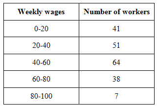
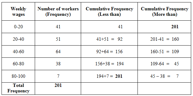
Solution: First, we make a cumulative frequency table:

Less than Ogive:

On the x-axis, mark the upper limits of class intervals and less than type cumulative frequencies are marked on the y-axis. For drawing less than ogive, plot the points (20, 41), (40, 92), (60, 156), (80, 194), (100, 201) on the graph paper and then join these points by freehand to obtain the less than ogive. 

Greater than Ogive or More than Ogive:

On the x-axis, mark the lower limits of class intervals and more (greater) than type cumulative frequencies are marked on the y-axis. For drawing more than ogive, plot the points (0, 201), (20, 160), (40, 109), (60, 45), (80, 7) on the graph paper and then join these points by freehand to obtain the more than ogive.

Both the two ogives (less than ogive and more than ogive) are shown in the following figure:

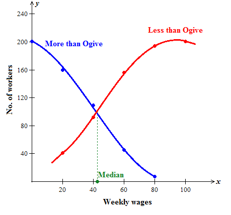
Determine the Median:

Draw a perpendicular line from the point of intersection of these curves on the x-axis. The point at which this perpendicular line meets the x-axis gives the median. Here, the median is 42.652.

(Source – Various books from the college library)

Copyrighted Material © 2019 - 2024 Prinsli.com - All rights reserved

All content on this website is copyrighted. It is prohibited to copy, publish or distribute the content and images of this website through any website, book, newspaper, software, videos, YouTube Channel or any other medium without written permission. You are not authorized to alter, obscure or remove any proprietary information, copyright or logo from this Website in any way. If any of these rules are violated, it will be strongly protested and legal action will be taken.